Tutorials

These set of tutorials provide more insight in the workings of LibKet for different commonly used quantum circuits, backends and advanced operations. All tutorial code can be found in the LibKet examples folder. If not mentioned otherwise, all expressions are evaluated for 1024 shots on all active backends. This section is complemantary material to the example code and as such the tutorials are best followed with code and documenation side to side.

Tutorial 1: Bell state

This tutorial shows how to create a simple LibKet expression, the Bell circuit.

Bell state circuit

Tutorial 2: Quantum Teleportation

This tutorial implements the quantum teleportation circuit, which teleports the state of the first qubit to the third qubit by using measurements taken from the first two qubits.

Quantum Teleportation circuit

Tutorial 3: Advanced

This tutorial shows the use of more advanced filters and gates to create this arbitrary circuit. The circuit itselfs serves no real purpose, but is rather an example of how LibKet handles filters and gate functors.

Advanced circuit

Tutorial 4: Static_for with graph

This tutorial shows how to implement the static_for function in combination with the LibKet graph class. Here the static_for loop is used to apply a cnot gate between every connected node in the graph. The ring graph with five nodes is represented as a list of edges. From this, it follows that the static_for loop should iterate over all edges in this list and apply a cnot function between two nodes that are connected, where the first node is the control and the second node the target qubit.

Static_for circuit

Tutorial 5: QPU execution

In this tutorial, three methods of retrieving QPU results are shown:

• Asynchronous execution

• Synchronous execution

• Evaluation

Both asynchronous and synchrounous execution return a pointer to the quantum job. The asynchronous option does not interrupt the code exection and the QPU execution will run in the background, so you can run code while the quantum expression is being evaluated. The synchronous option waits until the QPU has finished evaluating the quantum expression before contuing with the main code. For both methods, results can be retreived using the job->get() function.

The evaluation method is similar to the sychronous execution, but directly returns results in JSON format instead of the QObj pointer. The circuit belows shows the simple quantum expression used in this tutorial:

Simple quantum expression

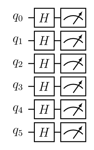
Tutorial 6: Quantum Fourier Transform

Here, the LibKet circuit QFT is used to construct a QFT circuit with allswap at the end. The Quantum Fourier Tranform. More information on the QFT can be found here. The inverse QFT can be applied by using the QFTdag() circuit.

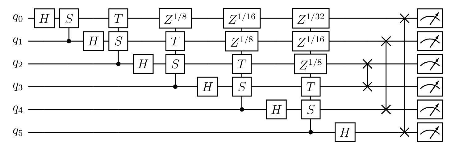
QFT circuit for 6 qubits

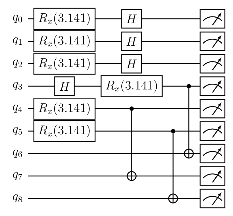
Tutorial 7: Arbitrary Control Circuit

The following circuit implements the arbitrary control circuit. It takes four parameters: A controlled binary gate, a filter for the control qubits, a filter for the ancilla qubits and a filter for the target qubit. This example implements a 4-qubit controlled X-gate. The first four qubits are used a control for the target qubit \(q_4\). For every \(N\) control qubits, \(N-1\) ancilla qubits are needed, in this case the last three qubits.

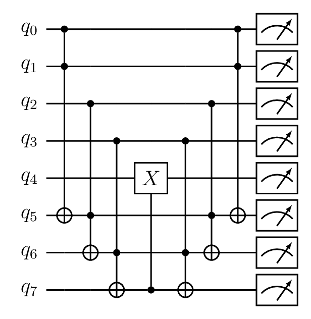
Arbitrary Control circuit for cnot gate

Tutorial 8: Allswap

The Allswap circuit creates a quantum expression where the qubit order in a given selection is flipped.

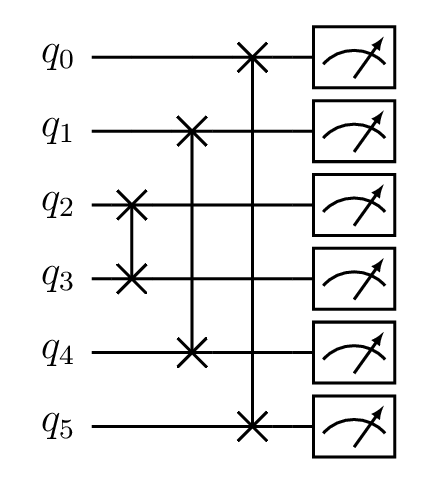
Allswap circuit

Tutorial 9: QAOA

This tutorial shows the implementation of a QAOA circuit for the Maximum Cut problem on arbitrary graph. More information on the QAOA can be found here. This toturial shows some more advance use of the static_for() function. The circuit is constructed for a singe QAOA iteration (\(p=1\)). This tutorial only shows how to create the QAOA circuit. For the QAOA to function, an classical optimizer is needed to optimize parameters \(\beta\) and \(\gamma\).

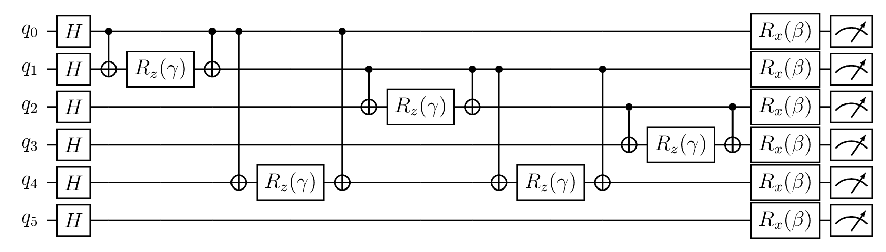
QAOA circuit for MaxCut

Tutorial 10: Hook

This tutorial illustrates the usage of the hook gate, which is able to reference another LibKet expression or create an expression from a cQASM string.

Circuit created with the Hook function

Tutorial 11: Just-In-Time Compilation

Using Just-In-Time Compilation, LibKet is able to use command line inputs for compile-time expresions. In this tutorial, a LibKet expression can be entered via the command line and will be processed later on in program.

Tutorial 12: Execution Scripts

he optional ftor_init, ftor_before, and ftor_after make it possible to inject user-defined code at three different locations of the execution process. In this tutorial, a simple statement after the execution collects the histogram data of the experiment using Qiskit’s get_count() function, generates a histogram plot and saves it to a file named ‘histogram.png’ in the build folder.

The init script imports the necessary packages for the qiksit visualization. After execution, the after script gets the counts and plots the histogram. It should be noted that the code injections are idented automatically and must not have trailing \t’s. Each line must end with \n.

Simple quantum expression for scripts tutorial

Tutorial 13: Unitary decomposition

This tutorial illustrates the basic usage of the built-in decomposition of a controlled 2x2 unitary gate into native gates. The unitary gate accepts an arbitrary 2x2 unitary matrix \(U\) as input and performs the ZYZ decomposition of \(U\). For example the following unitary matrix is used:

\[\begin{split}U = \frac{1}{\sqrt{2}} \begin{pmatrix} 1 & -1\\ 1 & 1 \end{pmatrix}\end{split}\]

The decomposition created the following quantum circuit:

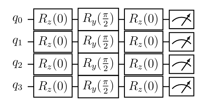
ZYZ decomposition of the unitary matrix

Tutorial 14: Controlled unitary decomposition

This tutorial implementes the controlled unitary decomposition, which is similar the the previous tutorial on the decomposed unitary. In this case, a control qubit is incluced to form a binary gate which controls the rotations of the unitary. For example the following unitary matrix is used:

\[\begin{split}U = \frac{1}{\sqrt{2}} \begin{pmatrix} 1 & -1\\ 1 & 1 \end{pmatrix}\end{split}\]

The controlled decomposition created the following quantum circuit:

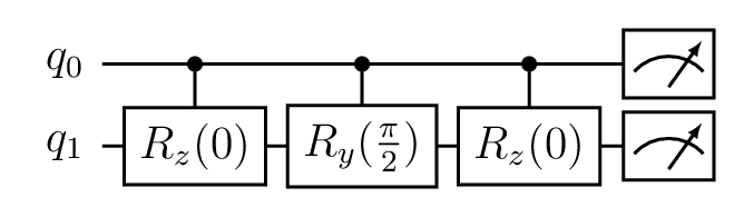
ZYZ decomposition of the unitary matrix

Tutorial 15: Quantum Program

The quantum program allows for a linear approach to constructing a quantum expression, as often seen in QASM languages. Here, qubit gates and operations are added sequantially and are translated to a quantum expression.

Circuit created by using the QProgram

Tutorial 16: HHL Algorithm

This tutorial shows the implementation of the Harrow-Hassidim-Lloyd (HHL) algorithm (see link). This algorithm is used to solve Linear systems of the form:

\[A \vec{x} = \vec{b}\]

where A is an \(N_{b}×N_{b}\) Hermitian matrix and \(\vec{x}\) and \(\vec{b}\) are \(N_b\)-dimensional vectors. In this example, \(A\) and \(\vec{b}\) are set to:

\[ \begin{align}\begin{aligned}\begin{split} A = \begin{pmatrix} 1 & -\frac{1}{3}\\ -\frac{1}{3} & 1 \end{pmatrix}\\\end{split}\\\begin{split}\vec{b} = \begin{pmatrix} 0 \\ 1\end{pmatrix}\end{split}\end{aligned}\end{align} \]

The controlled unitary evolution is computed to be:

\[\begin{split}U = e^{iAt} = e^{iA\frac{3\pi}{4}} = \frac{1}{2} \begin{pmatrix} -1+i & 1+i\\ 1+1 & -1+i \end{pmatrix}\\\end{split}\]

Which results in the following circuit example:

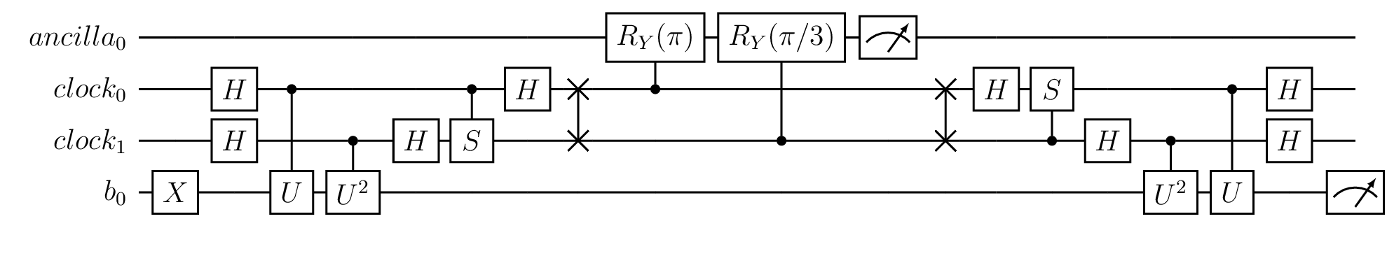
HHL Algorithm for a 2x2 matrix A and 2x1 vector b

The output result indeed confirms the expected ratio found in the HHL paper, which should be around \(prob(b_0)\) : \(prob(b_1)\) = 1 : 9.