Basics¶

The LibKet basiscs will cover the creation of simple generic quantum expressions, executing these expressions on different quantum backends and explaination of some quantum visualisation tools.

Generic Quantum Expressions¶

This section will cover the basics of creating a generic quantum expression in LibKet, selecting qubits with filters and applying gates to selected qubits. LibKet’s main components are

Filters
Gates
Circuits
Devices

Read this page for a quick overview of the different components.

Initialization¶

In order to work with an quantum expression, first an empty expression needs to be created. This can simply be done with:

auto expr = init();

Which creates an empty expression object. Notice that the number of qubits does not need to be specified yet and will be derived from the quantum device setup later.

Filters¶

Filters let you restrict the set of qubits to which an action such as a quantum gate or expression is applied. Filters operate relative to the input expression and can be combined to filter chains.

Filter functions¶

LibKet provides the following filter functions

all([expr]) resets all previous filters and selects all qubits
qubit<q>([expr]) selects the q-th qubits
qureg<q,length>([expr]) selects all qubits between q and q+length-1
range<qbegin,qend>([expr]) selects all qubits between qbegin and qend
select<q0,q1,...>([expr]) selects individual qubits q0, q1, …
shift<offset>([expr]) shifts the selected qubits by a positive or negative offset

For a detailed description check the Library.

Here and below [expr] means that the function can be called with and without an expression expr as will become clear from the following example.

Example

The following code snippet illustrates how to combine multiple filters to a filter chain that, though overly complicated, selects the first qubit. Note that counting starts at 0 as it is common practice in C/C++

auto f0 = select<0,4,2,6>(); // selects q0, q4, q2, q6
auto f1 = range<1,2>(f0);    // selects     q4, q2
auto f2 = qubit<1>(f1);      // selects         q2

Filter classes¶

An alternative way to create filters is by instantiating objects of filter classes and applying them using their operator().

Example

With this approach the above example code reads

auto f0 = QFilterSelect<0,4,2,6>();      // selects q0, q4, q2, q6
auto f1 = QFilterSelectRange<1,2>()(f0); // selects     q4, q2
auto f2 = QBit<1>()(f1);                 // selects         q2

Filter classes and functions can be combined since the functions are aliases that return an instance of the corresponding filter class.

Filter tags¶

The current selection can be saved using the tag<id>([expr]) function and restored at any later time via gototag<id>([expr]).

Example

auto f0 = select<0,4,2,6>(); // selects  q0, q4, q2, q6
auto f1 = tag<42>(f0);       // tags     q0, q4, q2, q6
auto f2 = range<1,2>(f1);    // selects      q4, q2
auto f3 = qubit<1>(f2);      // selects          q2
auto f4 = gototag<42>(f3);   // restores q0, q4, q2, q6

It is recommended to saveguard quantum expressions that should be usable as generic components in other expressions with a tag and restore the original selection on exit.

auto myexpression = gototag<42>( your-quantum-expression( tag<42>() ) );

The above expression can now be applied without changing the selection on return.

auto f0 = select<0,4,2,6>();
auto e0 = myexpression(f0);  // q0, q4, q2, q6 selected on return

Tags can be nested with different or same numbers. If multiple tag<id> s with the same id number are applied without a resolving gototag<id> then the next gototag<id> restores the selection of the ‘nearest’ tag<id>

auto f0 = all(tag<0>(range<1,2>(tag<0>(all()))));
auto f1 = gototag<0>(f0); // restores range<1,2>()

Filter Concatenations¶

Filters can be concatenated into a new filter by using thd << operator:

auto f0 = select<0,2>(); // selects q0, q2
auto f1 = select<1,3>(); // selects q1, q3
auto f2 = f0<<f1;        // selects q0, q2, q1, q3

Gates¶

Gates apply to all qubits of the current filter chain in a single-instruction multiple-data (SIMD) like fashion. That is, a single-qubit gate like the Hadamard (H) gate when applied to an \(n\)-qubit register is applied to each single qubit individually

\[H^{\otimes n}\lvert\psi\rangle = H\lvert\psi_0\rangle\otimes\cdots\otimes H\lvert\psi_{n-1}\rangle\]

Unary (One qubit) Gates¶

This gate set includes all one-qubit operations, such as Pauli operations, arbitrary rotations around the X-, Y- or Z-axis and measurements. Examples are:

auto e0 = h([expr]);            //Applies a Hadamard gate to all qubits in [expr]
auto e1 = rz([theta], [expr]);  //Applies a Z-rotation to all qubits in [expr] by angle [theta]

Binary (Two qubit) Gates¶

This gate set includes all two-gubit operations, such as CNOT, CPHASE or other controlled rotations. Examples are:

auto e0 = cnot(sel<0>(), sel<1>([expr]));            //CNOT gate on qubit 0 (control) and qubit 1 (target) in [expr]
auto e1 = cphase([theta], sel<0>(), sel<1>([expr])); //CPhase gate on qubit 0 (control) and qubit 1 (target) in [expr] by angle [theta]

Ternary (Three qubit) Gates¶

This gate set includes all three-gubit operations, such as the TOFFOLI gate:

auto e0 = ccnot(sel<0>(), sel<1>(), sel<2>([expr])); //Toffoli gate on qubit 0, 1 (control) and qubit 2 (target) in [expr]

Example¶

With this convention in mind we are ready to write our first quantum algorithm

auto e0 = init();
auto e1 = sel<0,2>(e0);
auto e2 = h(e1);
auto e3 = all(e2);
auto e4 = cnot(sel<0,2>(), sel<1,4>(e3));
auto e5 = measure(all(e4));

which corresponds to the following quantum circuit

Figure made with TikZ

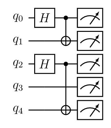
This image shows the circuit created with the above line of code

In LibKet we have provided as standard implementation of many of the quantum gates commonly used in quantum algorithms. For all gates, see the Library section Gates.

Circuits¶

Certain quantum circuits are used in the implementation of many quantum algorithms. To make it easier to implement large quantum algorithms some of these circuits are standardly implemented in LibKet. This way the user can create a large quantum circuit with just a single line of code!

Example: Quantum Fourier Transform

The code below can be used to apply the Quantum Fourier Transform on qubits 0 to n.

auto expr = qft(range<0,n>(init()));

This generates the following circuit for \(n = 5\):

Figure made with TikZ

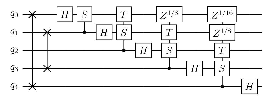
This image shows the circuit created with the above line of code

Apart from QFT LibKet also has a standard implementation of other quantum circuits. See section Circuits for all available circuits currently implemented in LibKet.

Devices¶

With the succesful creation of a quantum expression, it can now be executed on a quantum device. This is where the power of LibKet shows, by reinterpeting the generic quantum expression to a the device specific quantum assembly language. For all quantum devices see the Library section Devices.

A quantum device can be initialised with the QDevice<QDeviceType, Qubits> class. The generic quantum expression can then we loaded onto the device (Note: The number of qubits used in the quantum expression must not exceed the number of qubits set to the QDevice). Then the device can evaluate the quantum expression for a given number of shots. Here an example is given to evaluate a quantum expression on the QuEST simulator of 4 qubits for 2048 shots:

QQDevice<QDeviceType::quest, 4> device; // Initalize quantum device (QuEST simulator for 4 qubits)
device(expr);                           // Load generic quantum expression to device
device.eval(2048);                      // Evaluate the quantum kernel for 2048 shots

Result retrieval (Python based)¶

Retrieving the results differs slightly from device to device. For Python oriented backends (AQASM, Cirq, cQASM, OpenQASM, Quil) results put in a JSON object. The following code snippet shows how the result is loaded into a JSON object and results are printed to standard output:

utils::json result = device.eval(shots);
std::cout << "Job ID     : " << device.get<QResultType::id>(result)               << std::endl;
std::cout << "Time stamp : " << device.get<QResultType::timestamp>(result)        << std::endl;
std::cout << "Histogram  : " << device.get<QResultType::histogram>(result)        << std::endl;
std::cout << "Duration   : " << device.get<QResultType::duration>(result).count() << std::endl;
std::cout << "Best       : " << device.get<QResultType::best>(result)             << std::endl;

Alternatively, the entire content of the JSON object can be dumped to the output with:

std::cout << result << std::endl;          //Print without formatting
std::cout << result.dump(2) << std::endl;  //Use pretty print with indent 2

Result retrieval (QuEST & QX)¶

The QuEST and QX simulators can simulate the state of a quantum register and return an exact result of the qubit states. It can also determine the probabilities of a quantum states and simulate a measurement distribution. The following code print the results for a QuEST or QX device. An example output is given for \(H\lvert0\rangle\)

QuEST example:

auto expr = h(init());

//QuEST Simulator
QDevice<QDeviceType::quest, 1> quest;
quest(expr);
quest.eval(1);
std::cout << quest.reg()           << std::endl; //Returns exact quantum state
std::cout << quest.probabilities() << std::endl; //Returns probalities of quantum states
std::cout << quest.creg()          << std::endl; //Returns a classical measurement

Output:

--------------[quantum state]--------------
     (+0.70710678,+0.00000000) |0> +
     (+0.70710678,+0.00000000) |1> +
-------------------------------------------
0.500000000000000,0.500000000000000
0

QX example:

auto expr = h(init());

//QX Simulator
QDevice<QDeviceType::qx, 1> qx;
qx(expr);
qx.eval(1);
qx.reg().dump();  //Prints execution time, quantum state and measurement data

Output:

[+] executing circuit '' (1 iter) ...
[+] circuit execution time: 0.000235529 sec.
--------------[quantum state]--------------
  [p = +0.5000000]  (+0.7071068,+0.0000000) |0> +
  [p = +0.5000000]  (+0.7071068,+0.0000000) |1> +
-------------------------------------------
[>>] measurement averaging (ground state) :  | +0.00000000 |
-------------------------------------------
[>>] measurement prediction               :  |         X |
-------------------------------------------
[>>] measurement register                 :  |         0 |
-------------------------------------------

Visualization¶

The show() function

Filters and all other components generate an abstract syntax tree (AST) that represents the quantum expression. If you are interested how this AST looks like or you want to debug your expression use the show<depth>(expr) function. Only one level of the AST is printed by default.

Qasm2Circ

The qasm2tex_visualizer device can load an expression and output a LaTeX file which in combination with the xyqcirc.tex file can create a LaTeX image of the quantum circuit. Example:

QDevice<QDeviceType::qasm2tex_visualizer, nqubits> device;
device(expr);
device.to_file("filename");

Other LaTeX Parsers

The Qiskit, Cirq and IBMQ devices provide a LaTeX parser that can convert the quantum expression to a LaTeX code string. This string can then be printed to the standard output:

std::cout device.to_latex() << std::endl;

Terminal Visualisation

The Qiskit, Cirq and IBMQ devices also provide a terminal ASCII art visualisation of the quantum expression. This can be directly printed on the command-line interface, negating the need for a LaTeX interpreter

std::cout device.print_circuit() << std::endl;

Next read Components.